Quantum mechanical waves

Quantum mechanical waves

Main article: Schrödinger equation

See also: Wave function

The Schrödinger equation describes the wave-like behavior of particles in quantum mechanics. Solutions of this equation are wave functions which can be used to describe the probability density of a particle.

A propagating wave packet; in general, the envelope of the wave packet moves at a different speed than the constituent waves.^[28]

[edit]de Broglie waves

Main articles: Wave packet and Matter wave

Louis de Broglie postulated that all particles with momentum have a wavelength

where h is Planck's constant, and p is the magnitude of the momentum of the particle. This hypothesis was at the basis of quantum mechanics. Nowadays, this wavelength is called the de Broglie wavelength. For example, the electrons in a CRT display have a de Broglie wavelength of about 10⁻¹³ m.

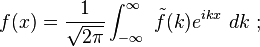
A wave representing such a particle traveling in the k-direction is expressed by the wave function as follows:

where the wavelength is determined by the wave vector k as:

and the momentum by:

However, a wave like this with definite wavelength is not localized in space, and so cannot represent a particle localized in space. To localize a particle, de Broglie proposed a superposition of different wavelengths ranging around a central value in a wave packet,^[29] a waveform often used in quantum mechanics to describe the wave function of a particle. In a wave packet, the wavelength of the particle is not precise, and the local wavelength deviates on either side of the main wavelength value.

In representing the wave function of a localized particle, the wave packet is often taken to have a Gaussian shape and is called a Gaussian wave packet.^[30] Gaussian wave packets also are used to analyze water waves.^[31]

For example, a Gaussian wavefunction ψ might take the form:^[32]

at some initial time t = 0, where the central wavelength is related to the central wave vector k₀ as λ₀ = 2π / k₀. It is well known from the theory of Fourier analysis,^[33] or from the Heisenberg uncertainty principle (in the case of quantum mechanics) that a narrow range of wavelengths is necessary to produce a localized wave packet, and the more localized the envelope, the larger the spread in required wavelengths. The Fourier transform of a Gaussian is itself a Gaussian.^[34] Given the Gaussian:

the Fourier transform is:

The Gaussian in space therefore is made up of waves:

that is, a number of waves of wavelengths λ such that kλ = 2 π.

The parameter σ decides the spatial spread of the Gaussian along the x-axis, while the Fourier transform shows a spread in wave vector k determined by 1/σ. That is, the smaller the extent in space, the larger the extent in k, and hence in λ = 2π/k.